Big-O Notation

Categorizes algorithms on time/memory based on input.

Why?

• Helps us make decisions on what data structures and algorithms to use.

Fundamental concept

As input grows, how fast does computation or memory grow?

Important concepts

Growth is with respect to input

fn sum_char_codes(input: String) -> u32 {
    let mut i = 0;
    for char in input.chars() {
        i += char as u32;
    }
    i
}

It runs an iteration in the for loop for the length of the string. This function has time complexity.

(Generally, look for loops to determine time complexity)

You always drop constants

While practically important, they're not theoretically important.

For example, if comparing and :

		(10x bigger)
		(100x bigger)
		(1000x bigger)

We're not concerned with the exact time, but instead, how it grows.

Practical and theoretical differences

Just because is faster than doesn't mean it's always better.

Remember, we drop constants. Therefore, is faster than but in the practical sense, it's slower for small inputs.

For example, in sorting algorithms, we use insertion sort for small inputs. Though slower in the theoretical sense because it's , it's faster in the practical sense because it's faster for small inputs than for example, quicksort which is .

Consider the worst-case scenario

fn sum_char_codes(input: String) -> u32 {
    let mut i = 0;
    for char in input.chars() {
        if char == 'E' { // checks if char is 'E', then instantly breaks
            return i;
        }
        i += char as u32;
    }
    i
}

This function still has time complexity because we're looking for the worst-case scenario.

While there are some algorithms where it's better to reason using the best case and the average case, most of the time, we're concerned with the worst-case scenario.

In interviews, almost always assume the worst-case scenario.

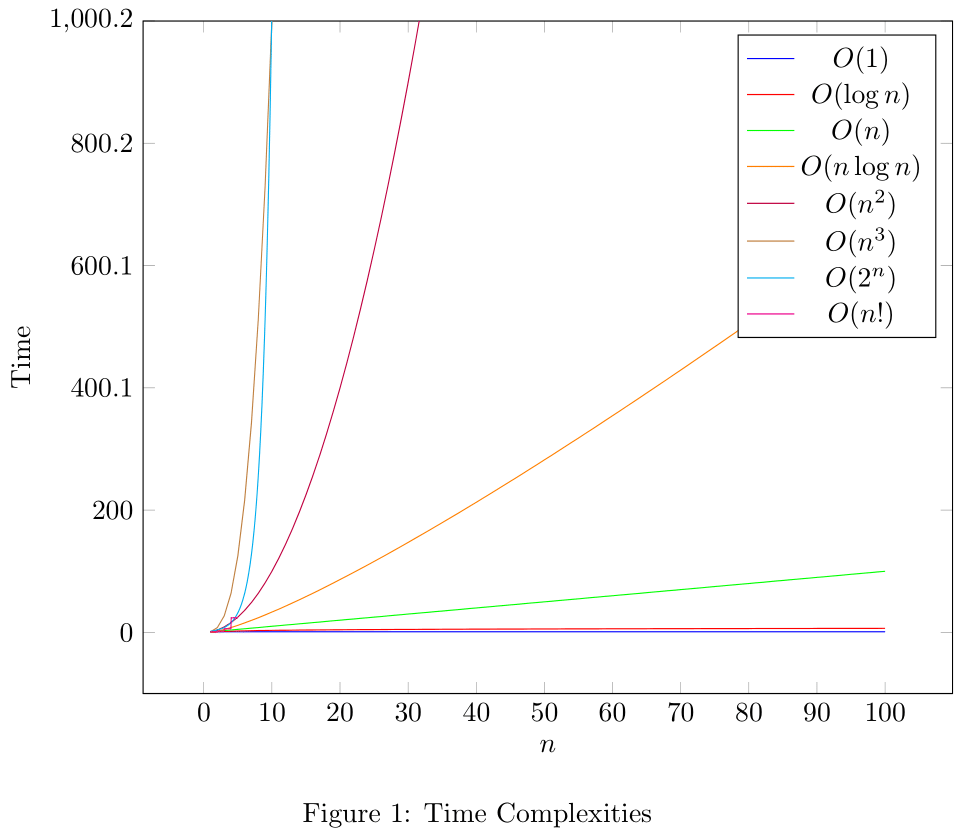
Common Big-O runtimes

Big-O	Name	Example	Notes
	Constant	Hash table lookup	Fastest
	Logarithmic	Binary search	Fast
	Linear	Simple search	Slow
	Log-linear	Quicksort	Fast
	Quadratic	Selection sort	Slow
	Cubic	Matrix multiplication	Slow
	Exponential	Traveling salesperson	Very slow
	Factorial	Traveling salesperson	Very slow

Simple examples

fn sum_char_codes(input: String) -> u32 {
    let mut i = 0;
    for char in input.chars() { // loop 1
        for char in input.chars() { // loop 2
            i += char as u32;
        }
    }
    i
}

For each character in the string, we iterate through the string again. This is .

fn sum_char_codes(input: String) -> u32 {
    let mut i = 0;
    for char in input.chars() { // loop 1
        for char in input.chars() { // loop 2
            for char in input.chars() { // loop 3
                i += char as u32;
            }
        }
    }
    i
}

Just like the previous example, but we iterate through the string three times. This is .

(Quicksort) - will be covered in a later section.

Binary search trees.

This is a very unique time complexity.

Other notations

is the lower bound of an algorithm.

For example, means that the algorithm will take at least time.

is the tight bound of an algorithm.

For example, means that the algorithm will take at least time and at most time.

Space complexity

Space complexity is the amount of memory an algorithm takes up. Generally it's less consequential than time complexity.

return <Component {...props} /> // O(n) time and O(n) space

Conclusion

• Big-O is a way to categorize algorithms based on time/memory.
• Growth is with respect to input.
• You always drop constants.
• In most cases consider the worst-case scenario.